Chapter 4 Exploratory data analysis
4.1 Histogram
Rn
hist(InRn$Rn,
       prob = T,
       col = "red",
       breaks = 10,
       main = "Histogram Indoor Radon",
       xlab = expression("Rn " * "[Bq" * m^-3 * "]"))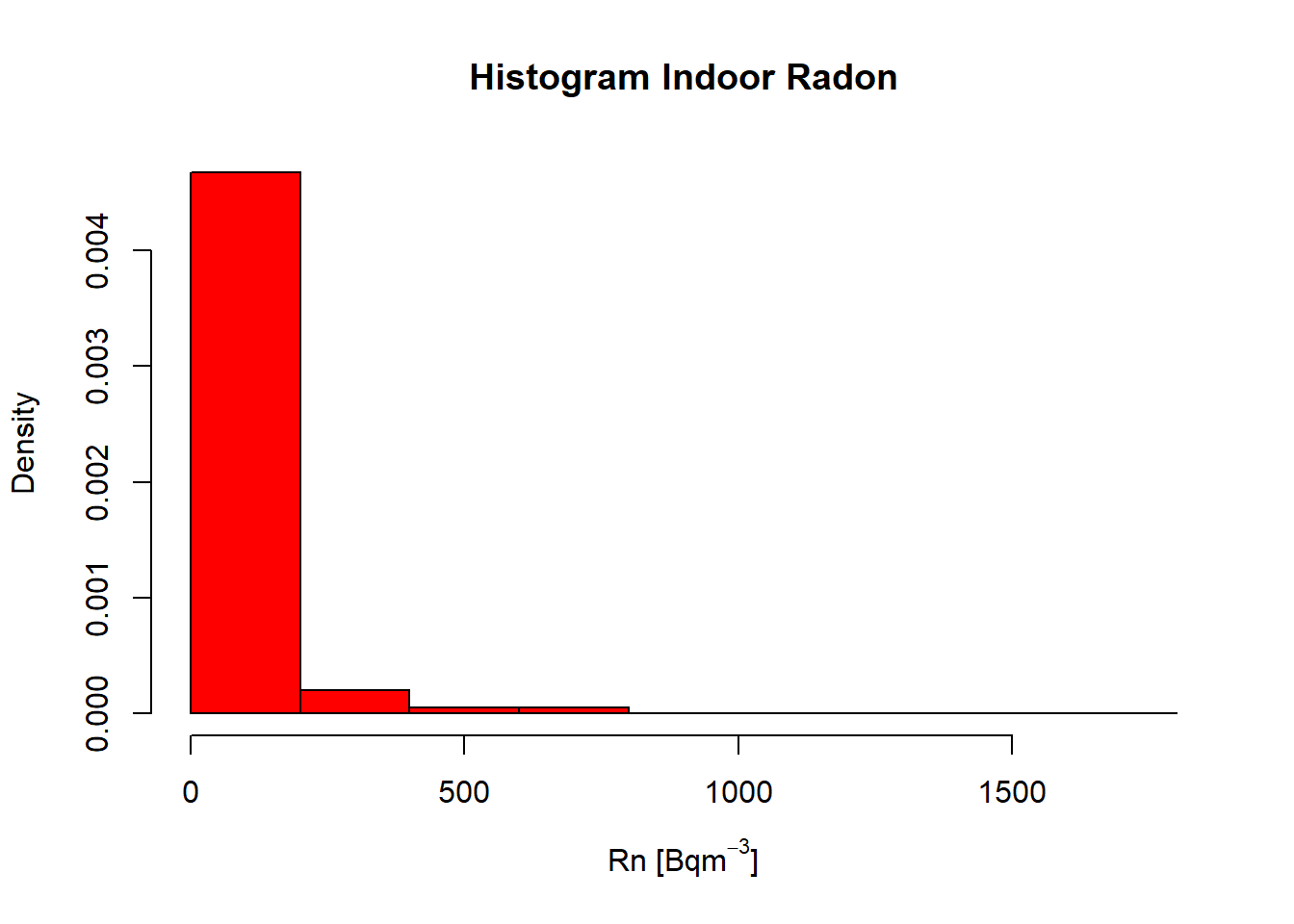
  StatDA::qqplot.das(InRn$Rn,
             distribution = "norm",
             col = 1, envelope = 0.95,
             datax = T,
             main = "Q-Q plot (InRn)")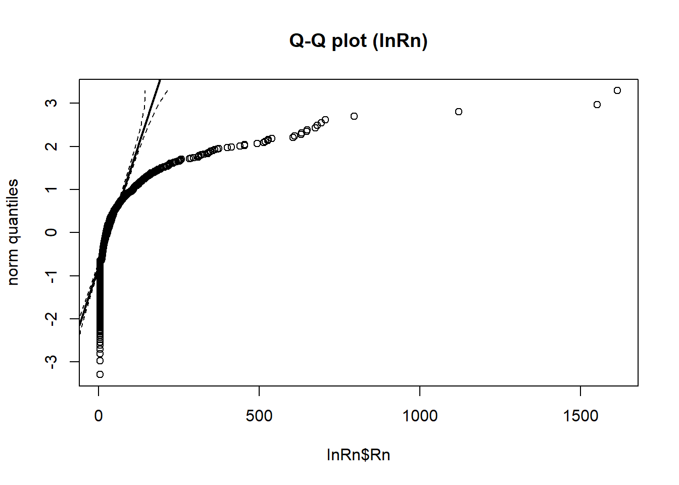
## Box-Cox transformation ----
  BCT <- MASS::boxcox(InRn$Rn ~ 1, lambda = seq(-1, 1, 1/100))
  title("Box-Cox Transformation")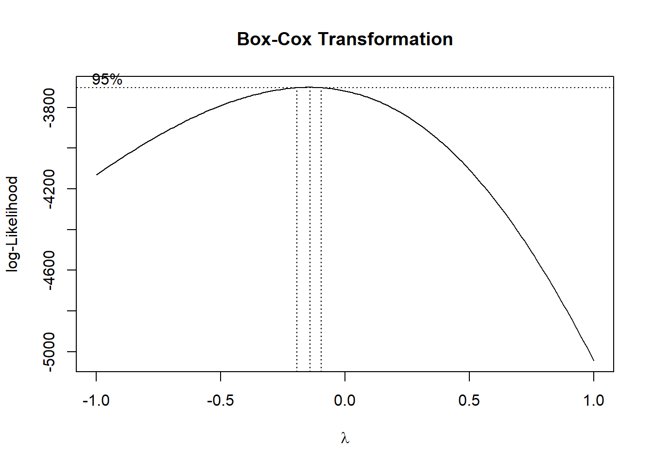
  BCT <- as.data.frame(BCT)
  # lambda <- BCT[BCT$y == max(BCT$y), ]$x # -0.17
  # InRn$BCT <- (InRn$Rn^lambda-1)/lambda
  lambda <- 0
  InRn$LogRn <- log(InRn$Rn)
## Histogram (logRn) ----
hist(InRn$LogRn,
col = "red",
breaks = 30,
prob = T,
main = "Histogram Indoor Radon",
xlab = expression("LogRn " * "[Bq" * m^-3 * "]"))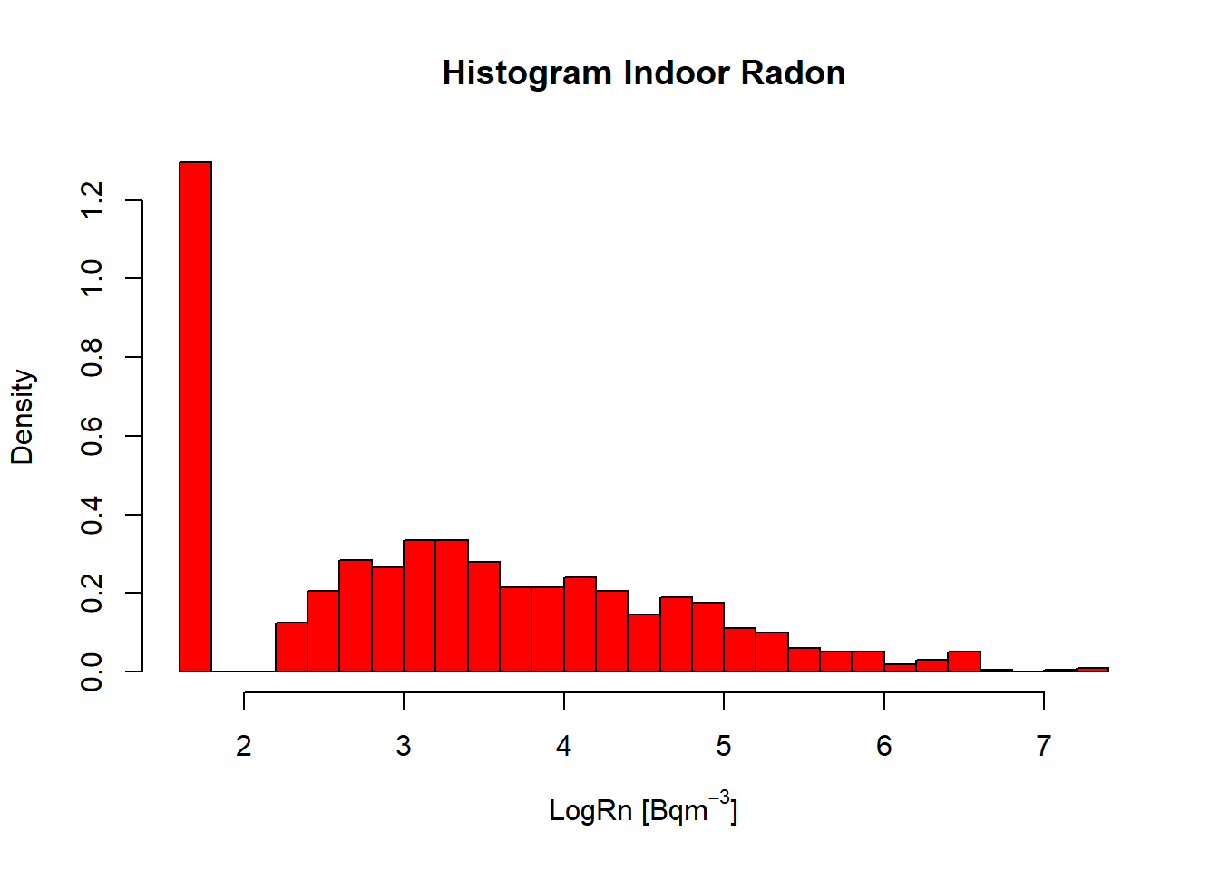
StatDA::qqplot.das(InRn$LogRn, distribution = "norm", col = 1, envelope = 0.95,datax=T, main = "Q-Q plot (log InRn)")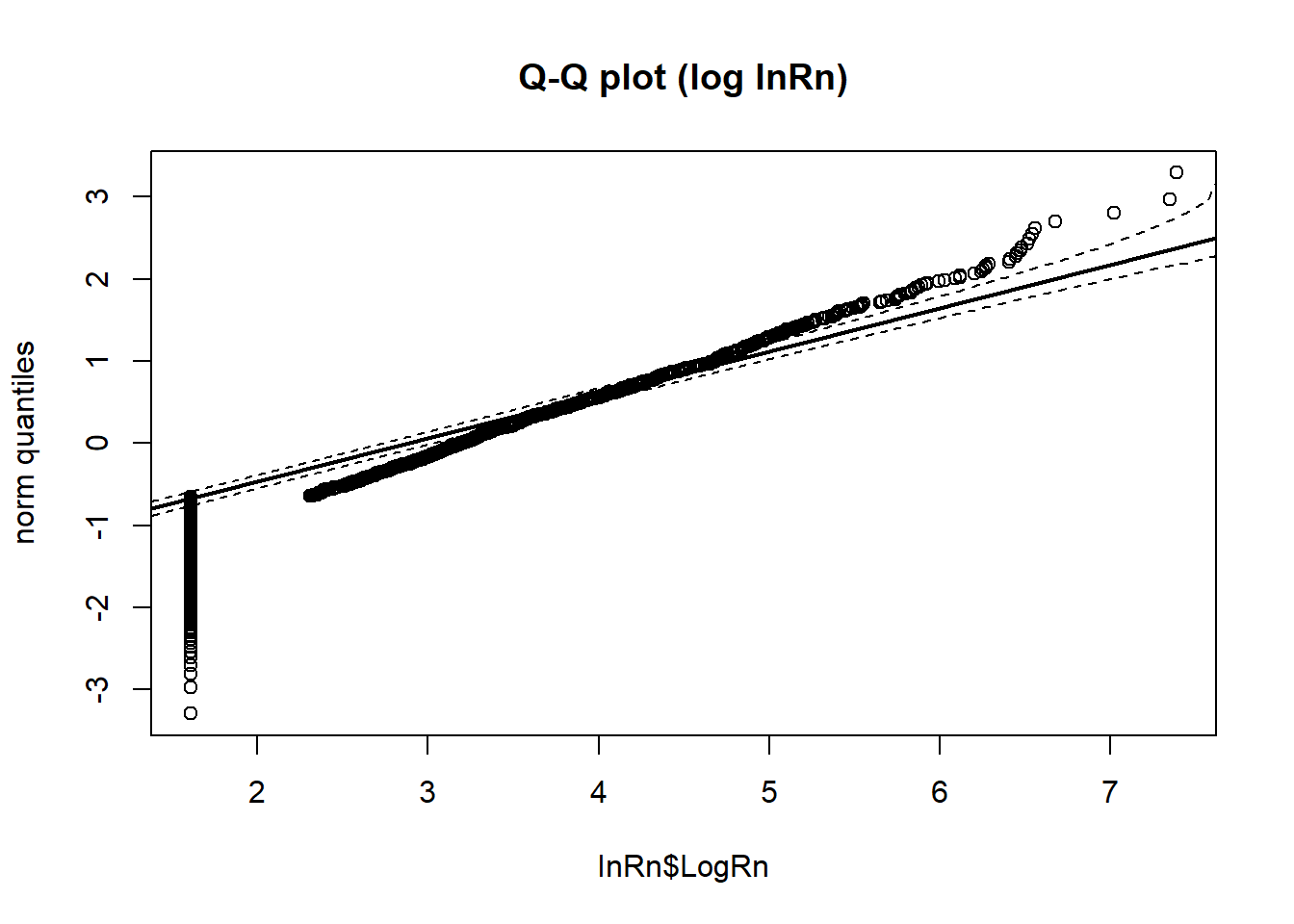
4.2 Missing data
Imputation of values below the detection limit
## ROS: “ROBUST” IMPUTATION METHOD ----
  DL <- 10
  InRn_DL <- InRn
  InRn_DL$Rn_Cen <- "FALSE"
  InRn_DL[InRn_DL$Rn <= DL,]["Rn_Cen"] <- "TRUE"
  InRn_DL$Rn_Cen <- as.logical(InRn_DL$Rn_Cen)
  ROS <- NADA::ros(InRn_DL$Rn, InRn_DL$Rn_Cen, forwardT = "log")
  ROS <- as.data.frame(ROS)
  # Replace Dl by the modeled values
  InRn_DL[InRn_DL$Rn_Cen == "TRUE",]["Rn"] <- ROS[ROS$censored == "TRUE",]["modeled"]
  InRn_DL$LogRn <- log(InRn_DL$Rn)
## q-q plots ----
par(mfrow=c(1,2))
StatDA::qqplot.das(InRn$LogRn,
distribution = "norm",
col = 1,
envelope = 0.95,
datax = T,
main = "Original data")
StatDA::qqplot.das(InRn_DL$LogRn,
distribution = "norm",
col = 1,
envelope = 0.95,
datax = T,
main = "After ROS")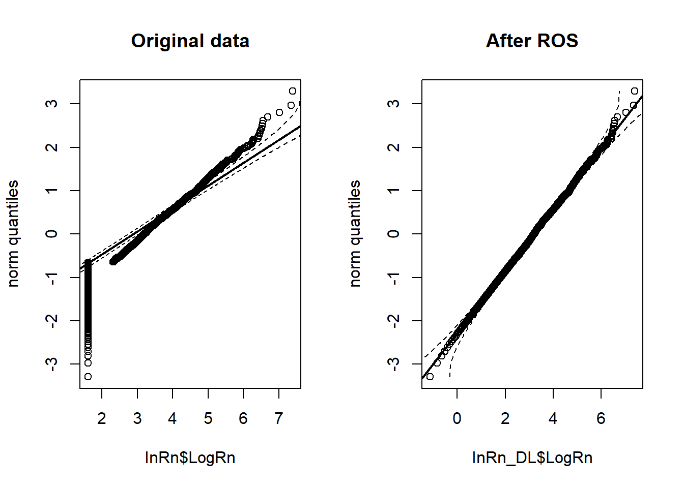
mean(InRn$Rn)# [1] 64.1 sd(InRn$Rn) # [1] 126 exp(mean(InRn$LogRn))# [1] 25.7 exp(sd(InRn$LogRn))# [1] 3.68 RL <- 200 # Bq m-3
100*(1 - pnorm(log(RL), mean = mean(InRn$LogRn), sd = sd(InRn$LogRn)))# [1] 5.8 mean(InRn_DL$Rn)# [1] 64.1 sd(InRn_DL$Rn) # [1] 126 exp(mean(InRn_DL$LogRn))# [1] 24.8 exp(sd(InRn_DL$LogRn))# [1] 4.04 100*(1-pnorm(log(RL), mean = mean(InRn_DL$LogRn), sd = sd(InRn_DL$LogRn)))# [1] 6.74## Histogram (logRn) ----
par(mfrow=c(1,2))
hist(InRn$LogRn,
col = "red",
breaks = 30,
prob = T,
ylim = c(0, 0.5),
main = "Origical data",
xlab = expression("LogRn " * "[Bq" * m^-3 * "]"))
hist(InRn_DL$LogRn,
col = "red",
breaks = 30,
prob = T,
ylim = c(0, 0.5),
main = "After ROS",
xlab = expression("LogRn " * "[Bq" * m^-3 * "]"))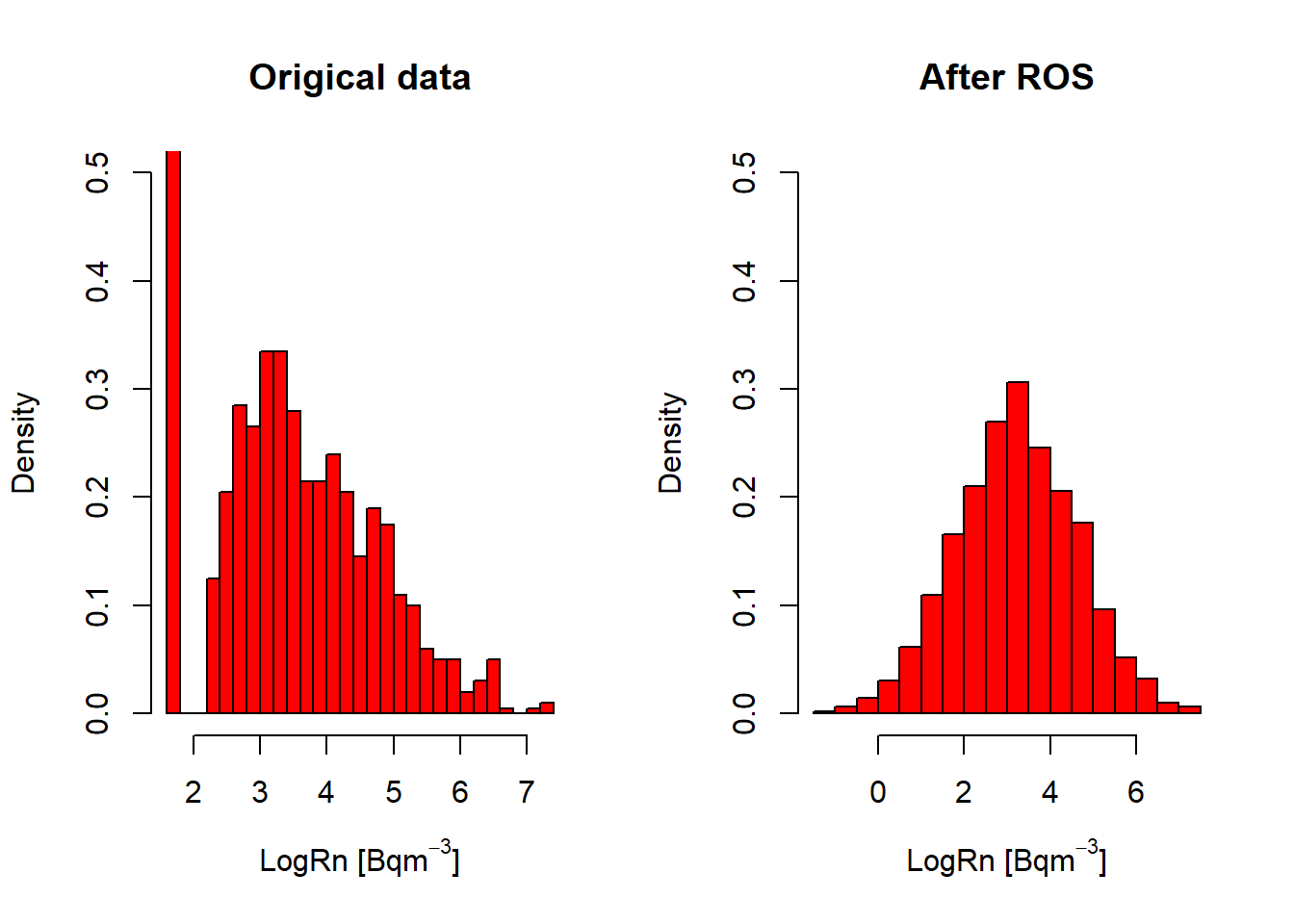
## Histogram, boxplot, q-q plot ----
  par(mfrow = c(1,3))
  hist(InRn_DL$LogRn,
       col = "red",
       breaks = 30,
       prob = T,
       main = "Histogram",
       xlab = expression("LogRn " * "[Bq" * m^-3 * "]"))
  lines(density(InRn_DL$LogRn), lwd = 1)

  boxplot(InRn_DL$LogRn,
          notch = TRUE,
          col=2,
          varwidth = TRUE,
          main = "Boxplot",
          ylab = "Lognormal transformation",
          xlab = expression("LogRn " * "[Bq" * m^-3 * "]"))

  StatDA::qqplot.das(InRn_DL$LogRn,
             distribution = "norm",
             col = 1,
             envelope = 0.95,
             datax = T,
             ylab = "Observed Value",
             xlab = "Expected Normal Value",
             main = ("Normal Q-Q plot"),
             line = "quartiles",
             pch = 3,
             cex = 0.7,
             xaxt = "s")
4.3 Spatial distribution
## Plot InRn measurements in Bq/m3 (with ggplot2) ----
  P_Rn <- ggplot() +
    geom_sf(data = Grids_10km) +
    geom_sf(data = InRn_DL, aes(color = Rn)) +
    scale_color_gradient(name = "Bq/m3", low = "blue", high = "red") +
    ggtitle("Indoor radon measurements (Simulated)")
  P_Rn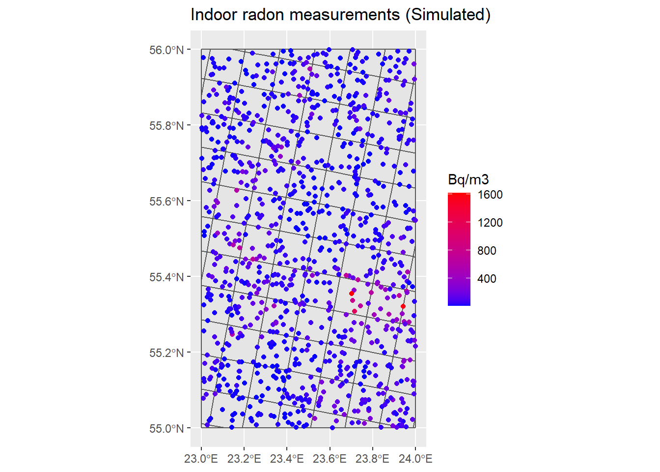
## Change intervale in the Rn scale ----
  breaks <- c(0, 50, 100, 200, 300, 500, max(InRn_DL$Rn))
  InRn_DL <- InRn_DL %>% mutate(brks = cut(Rn, breaks, include.lowest = T, right = F))
  cols <- colorRampPalette(c("blue", "red"))(6)
  # cols <- terrain.colors(6)
  # cols <- heat.colors(6, alpha = 1)
  # cols <- colorRampPalette(c("yellow", "red"))(6)
  P_Rn_brks <- ggplot() +
    geom_sf(data = Grids_10km) +
    geom_sf(data = InRn_DL, aes(fill = brks, color = brks)) +
    scale_fill_manual(name = "Bq/m3", values = cols, guide = guide_legend(reverse = TRUE)) +
    scale_color_manual(name = "Bq/m3", values = cols, guide = guide_legend(reverse = TRUE)) +
    ggtitle("Indoor radon measurements (Simulated)")
  P_Rn_brks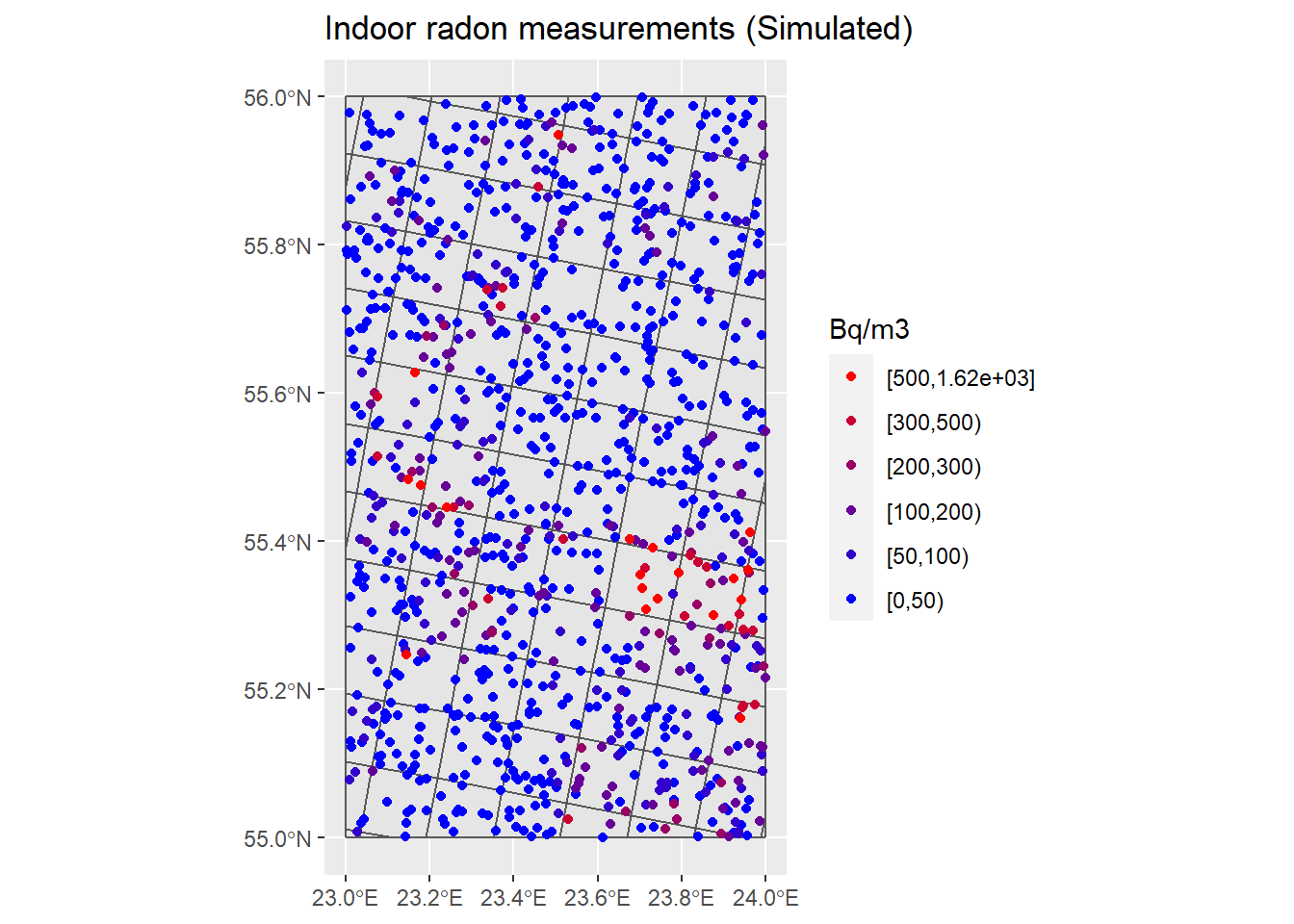
## Plot if Rn is higher than Reference level (1) or not (0) ----
  # Transform InRn to: 1 if Rn >= RL or 0 if Rn < RL ("Case")
    RL <- 200 # Bq m-3
    InRn_DL <- InRn_DL %>% mutate(Case = as.factor(ifelse(Rn >= 200, yes = 1, no = 0)))

    P_Cases <- ggplot() +
      geom_sf(data = Grids_10km) +
      geom_sf(data = InRn_DL, aes(fill = Case, color = Case)) +
      scale_fill_manual( name = "Bq/m3", labels = c("< 200",">= 200"), values = c("lightgreen", "red")) +
      scale_color_manual(name = "Bq/m3", labels = c("< 200",">= 200"), values = c("lightgreen", "red")) +
      # theme(legend.position = "none") +
      ggtitle("Indoor radon measurements (Simulated)")
    P_Cases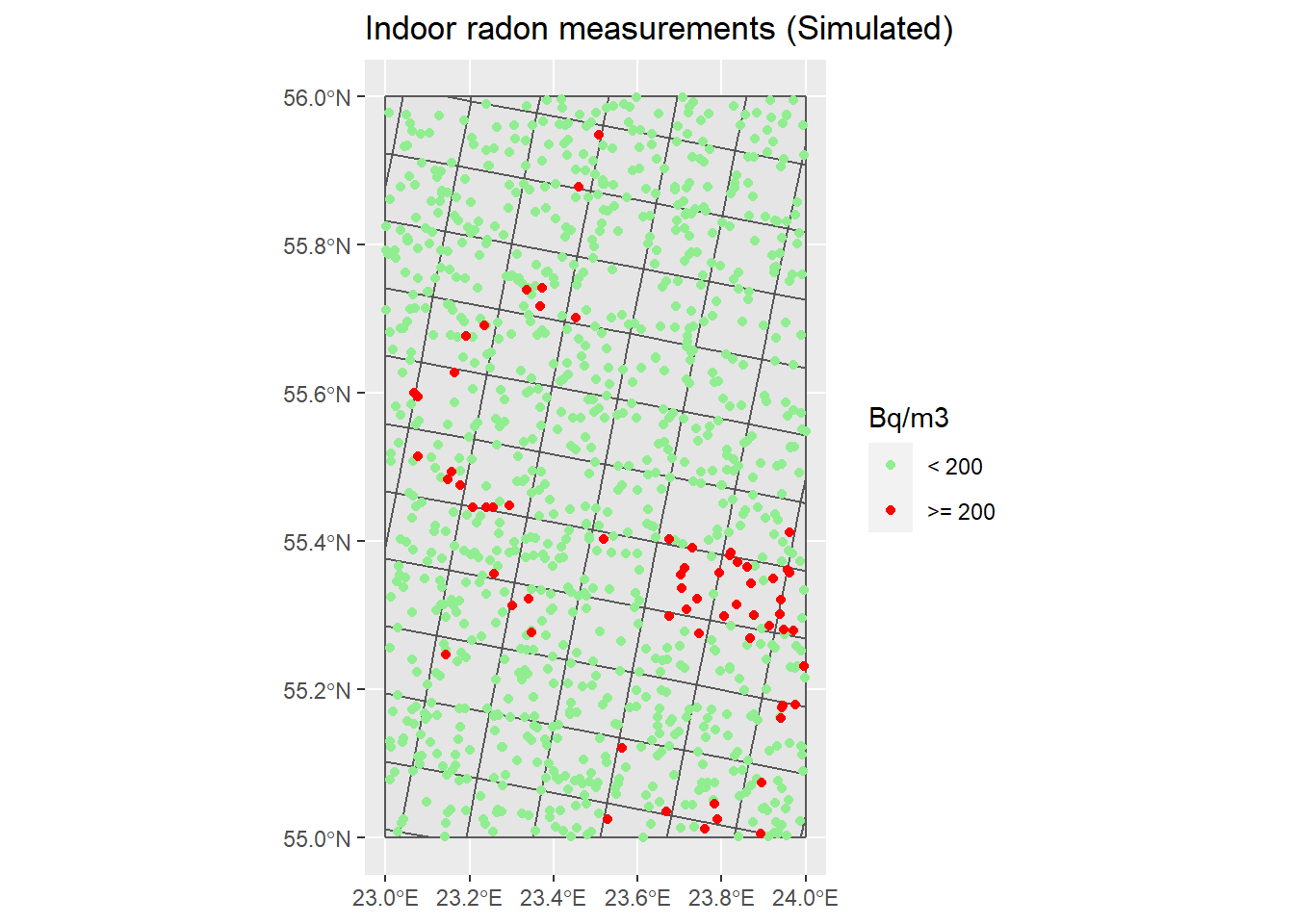
## Kernel density plots ----
  # The resulting density map is “noisier” for small bandwidth (h)
  # and “smoother” for large bandwidth (h).
  # A rule-of-thumb for an optimal value is h ≈ max(sx, sy)*0.7*n^-0.2
  # where n is the number of points,
  # and sx and sy the standard deviations of x- and y- coordinates of the points
  # See printed version of the EU Atlas for further information (in progress)
  # 2.4. Statistics, measurements, maping (part wirtten by P. Bossew)

  # All dwelling sampled (e.g. for detecting possible clusters; avoid overplotting)
    H <- st_coordinates(InRn_DL)
    h <- max(sd(H[,"X"]), sd(H[,"Y"])) * 0.7 * nrow(H)^-0.2
    KP_all <- InRn_DL %>%
      st_coordinates() %>%
      as_tibble() %>%
      ggplot() +
      geom_sf(data = Grids_10km) +
      stat_density_2d(aes(X, Y, fill = ..level.., alpha = ..level..),
                      h = h,
                      geom = "polygon") +
      scale_fill_distiller(palette = "Spectral") +
      theme(legend.position = "none") +
      #geom_sf(data = InRn_DL, size = .1) +
      ggtitle("Kernel density plots (all data)") +
      labs(x = "", y = "")
    KP_all
# Only dwellings with InRn > RL (cases == 1)
    H <- st_coordinates(filter(InRn_DL, Case == 1))
    h <- max(sd(H[,"X"]), sd(H[,"Y"])) * 0.7 * nrow(H)^-0.2
    KP_Cases <- InRn_DL %>% filter(Case == 1) %>%
      st_coordinates() %>%
      as_tibble() %>%
      ggplot() +
      geom_sf(data = Grids_10km) +
      stat_density_2d(aes(X, Y, fill = ..level.., alpha = ..level..),
                      h = h,
                      geom = "polygon") +
      scale_fill_distiller(palette = "Spectral") +
      theme(legend.position = "none") +
      geom_sf(data = filter(InRn_DL, Case == 1), size = .1) +
      ggtitle("Kernel density plots (InRn >= 200 Bq/m3)") +
      labs(x = "", y = "")
    KP_Cases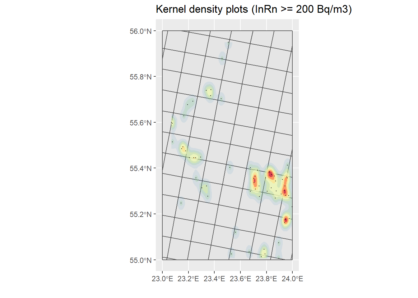
# Only dwellings with InRn < RL (cases)
    H <- st_coordinates(filter(InRn_DL, Case == 0))
    h <- max(sd(H[,"X"]), sd(H[,"Y"])) * 0.7 * nrow(H)^-0.2
    KP_No_Cases <- InRn_DL %>% filter(Case == 0) %>%
      st_coordinates() %>%
      as_tibble() %>%
      ggplot() +
      geom_sf(data = Grids_10km) +
      stat_density_2d(aes(X, Y, fill = ..level.., alpha = ..level..),
                      h = h,
                      geom = "polygon") +
      scale_fill_distiller(palette = "Spectral") +
      theme(legend.position = "none") +
      geom_sf(data = filter(InRn_DL, Case == 0), size = .1) +
      ggtitle("Kernel density plots (InRn < 200 Bq/m3)") +
      labs(x = "", y = "")
    KP_No_Cases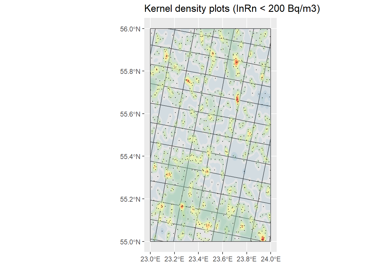
# Plot two (or more) figures in one
    library(gridExtra)
    grid.arrange(KP_No_Cases, KP_Cases, nrow = 2)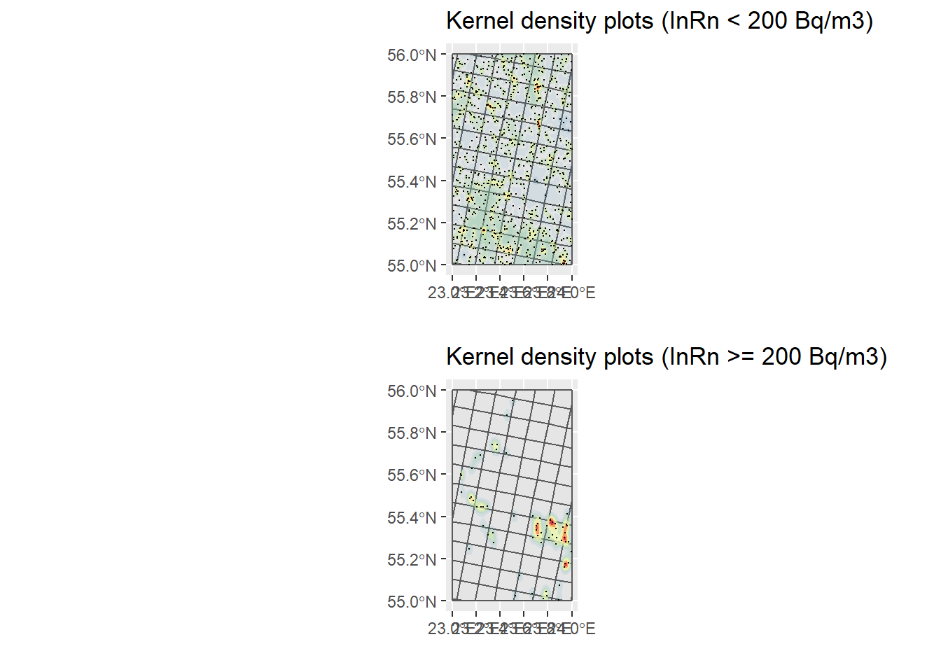
grid.arrange(KP_No_Cases, KP_Cases, nrow = 1)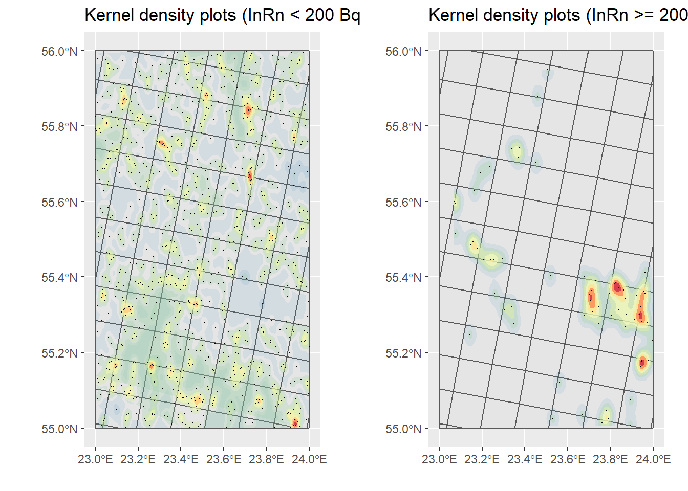
# InRn vs Geologia ----
  P_BG <- ggplot() +
      geom_sf(data = Country) +
      geom_sf(data = IGME5000,  aes(fill = AgeName), colour = NA) +
      geom_sf(data = InRn_DL, aes(), colour = 1, cex = 0.8) +
      scale_color_gradient(low = "blue", high = "red") +
      ggtitle("Geology 1:1M")
  P_BG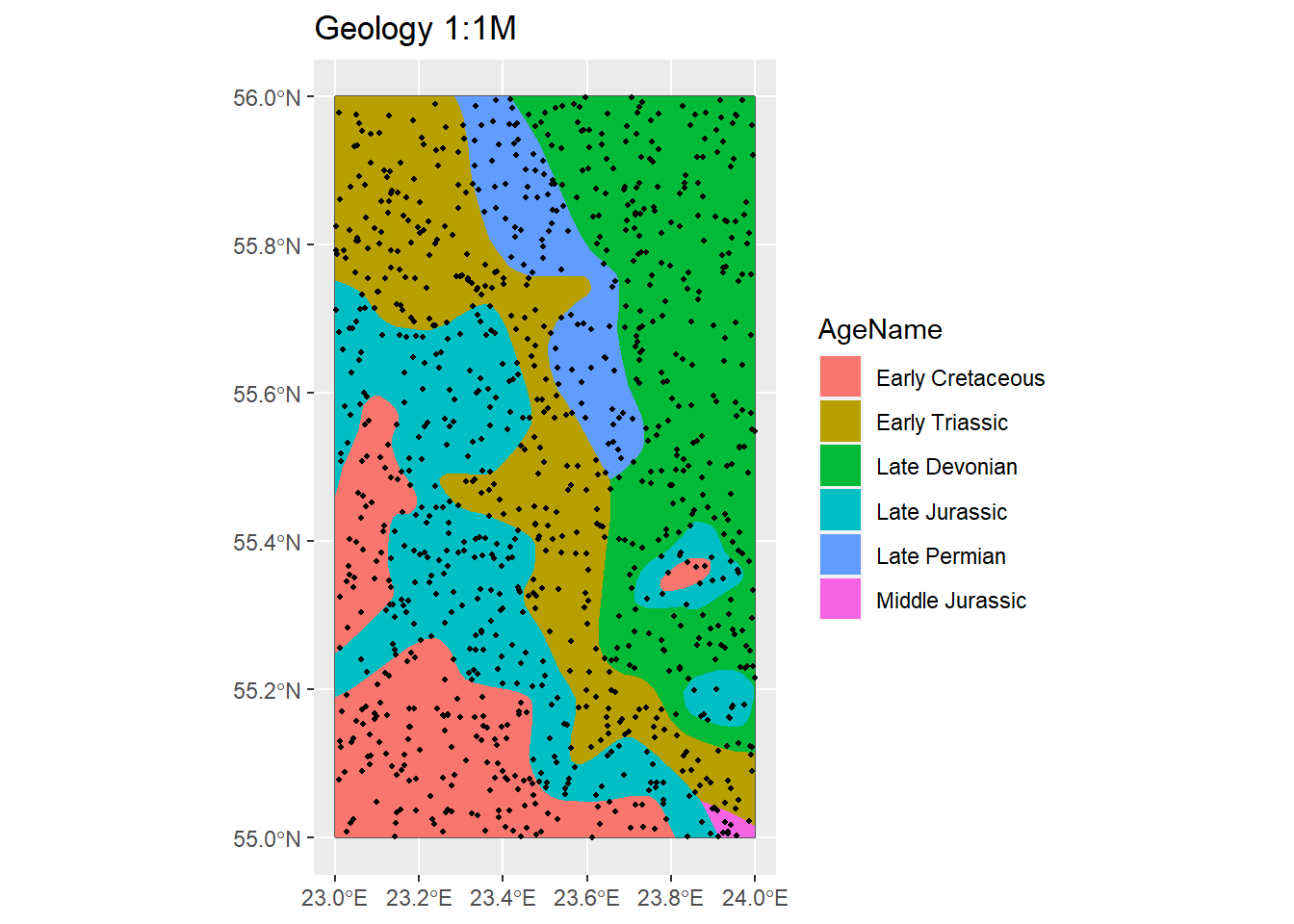
## Intersect ----
  InRn_DL_BG <- st_intersection(InRn_DL, IGME5000)
## Boxplots ----
par(mar = c(9,5,3,0.5), oma = c(0, 0.5, 0.5, 0.5), mfrow = c(1,1))
boxplot(LogRn ~ AgeName, InRn_DL_BG, col = 2,
varwidth = TRUE,
notch = T,
las = 2,
ylab = expression("LogRn " * "[Bq" * m^-3 * "]"),
xlab = "",
main = "Geology (AgeName)")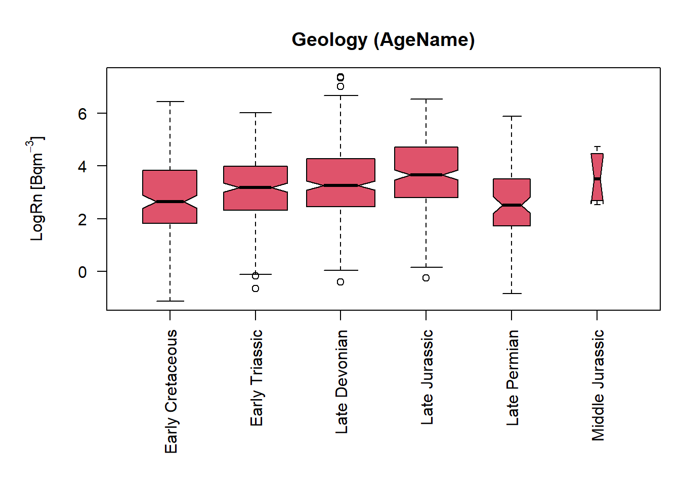
# ANOVA ----
  lm_BG <- lm(LogRn ~ AgeName, InRn_DL_BG)
  summary(lm_BG)
#
# Call:
# lm(formula = LogRn ~ AgeName, data = InRn_DL_BG)
#
# Residuals:
# Min 1Q Median 3Q Max
# -3.952 -0.904 -0.029 0.974 4.048
#
# Coefficients:
# Estimate Std. Error t value Pr(>|t|)
# (Intercept) 2.822 0.104 27.19 <2e-16 ***
# AgeNameEarly Triassic 0.255 0.136 1.87 0.0617 .
# AgeNameLate Devonian 0.517 0.133 3.90 0.0001 ***
# AgeNameLate Jurassic 0.859 0.137 6.28 5e-10 ***
# AgeNameLate Permian -0.247 0.184 -1.34 0.1793
# AgeNameMiddle Jurassic 0.767 0.464 1.65 0.0986 .
# ---
# Signif. codes: 0 '***' 0.001 '**' 0.01 '*' 0.05 '.' 0.1 ' ' 1
#
# Residual standard error: 1.36 on 994 degrees of freedom
# Multiple R-squared: 0.0613, Adjusted R-squared: 0.0566
# F-statistic: 13 on 5 and 994 DF, p-value: 2.89e-12 anova(lm_BG)# Analysis of Variance Table
#
# Response: LogRn
# Df Sum Sq Mean Sq F value Pr(>F)
# AgeName 5 120 23.92 13 2.9e-12 ***
# Residuals 994 1830 1.84
# ---
# Signif. codes: 0 '***' 0.001 '**' 0.01 '*' 0.05 '.' 0.1 ' ' 1