Summary statistics
  ## InRn by grids of 10 x 10 km (summry: N, AM, SD, GM, GSD) ----
  InRn_DL <- st_intersection(InRn_DL, Grids_10km)
  str(InRn_DL)
# Classes 'sf' and 'data.frame':    1000 obs. of  12 variables:
#  $ Rn       : num  5.113 0.785 1.763 6.323 36.349 ...
#  $ LogRn    : num  1.632 -0.242 0.567 1.844 3.593 ...
#  $ Rn_Cen   : logi  TRUE TRUE TRUE TRUE FALSE FALSE ...
#  $ brks     : Factor w/ 6 levels "[0,50)","[50,100)",..: 1 1 1 1 1 4 1 3 2 1 ...
#  $ Case     : Factor w/ 2 levels "0","1": 1 1 1 1 1 2 1 1 1 1 ...
#  $ CELLCODE : chr  "10kmE512N372" "10kmE513N367" "10kmE513N367" "10kmE513N367" ...
#  $ EOFORIGIN: num  5120000 5130000 5130000 5130000 5130000 5130000 5130000 5130000 5130000 5130000 ...
#  $ NOFORIGIN: num  3720000 3670000 3670000 3670000 3680000 3680000 3680000 3680000 3680000 3690000 ...
#  $ Id       : Factor w/ 1022 levels "1","2","3","4",..: 341 362 362 362 363 363 363 363 363 364 ...
#  $ GID_0    : chr  "LTU" "LTU" "LTU" "LTU" ...
#  $ NAME_0   : chr  "Lithuania" "Lithuania" "Lithuania" "Lithuania" ...
#  $ geometry :sfc_POINT of length 1000; first list element:  'XY' num  23 56
#  - attr(*, "sf_column")= chr "geometry"
#  - attr(*, "agr")= Factor w/ 3 levels "constant","aggregate",..: NA NA NA NA NA NA NA NA NA NA ...
#   ..- attr(*, "names")= chr [1:11] "Rn" "LogRn" "Rn_Cen" "brks" ...
  InRn_DL$Case <- as.numeric(as.character(InRn_DL$Case))

  InRn_Summary_Grids10km <- InRn_DL %>%
    group_by(Id) %>%
    summarize(N = n(),
              Case = sum(Case),
              AM = mean(Rn),
              SD = sd(Rn),
              GM = exp(mean((LogRn))),
              GSD = exp(sd(LogRn)),
              MIN = min(Rn),
              MAX = max(Rn))

  ## Add summary to grids of 10x10 km ----
  Grids_10km_Sum <- left_join(Grids_10km %>% as.data.frame(), InRn_Summary_Grids10km %>% as.data.frame(), by = "Id")
  Grids_10km_Sum <- Grids_10km_Sum %>%
    st_sf(sf_column_name = "geometry.x") %>%
    mutate(N = replace_na(N, 0))
  summary(Grids_10km_Sum)
#    CELLCODE           EOFORIGIN         NOFORIGIN             Id        GID_0              NAME_0
#  Length:93          Min.   :5120000   Min.   :3610000   340    : 1   Length:93          Length:93
#  Class :character   1st Qu.:5150000   1st Qu.:3640000   341    : 1   Class :character   Class :character
#  Mode  :character   Median :5160000   Median :3670000   361    : 1   Mode  :character   Mode  :character
#                     Mean   :5163871   Mean   :3674516   362    : 1
#                     3rd Qu.:5180000   3rd Qu.:3710000   363    : 1
#                     Max.   :5210000   Max.   :3740000   364    : 1
#                                                         (Other):87
#        N             Case            AM            SD            GM           GSD            MIN
#  Min.   : 0.0   Min.   :0.00   Min.   :  3   Min.   :  1   Min.   :  2   Min.   :1.12   Min.   :  0.3
#  1st Qu.: 7.0   1st Qu.:0.00   1st Qu.: 19   1st Qu.: 19   1st Qu.: 11   1st Qu.:2.28   1st Qu.:  1.7
#  Median :12.0   Median :0.00   Median : 39   Median : 39   Median : 24   Median :2.75   Median :  4.2
#  Mean   :10.8   Mean   :0.77   Mean   : 69   Mean   : 68   Mean   : 45   Mean   :2.95   Mean   : 11.4
#  3rd Qu.:14.0   3rd Qu.:1.00   3rd Qu.: 86   3rd Qu.: 77   3rd Qu.: 54   3rd Qu.:3.44   3rd Qu.: 11.3
#  Max.   :22.0   Max.   :9.00   Max.   :687   Max.   :549   Max.   :472   Max.   :6.20   Max.   :143.2
#                 NA's   :7      NA's   :7     NA's   :11    NA's   :7     NA's   :11     NA's   :7
#       MAX               geometry.x              geometry.y
#  Min.   :   5   POLYGON      :93   GEOMETRYCOLLECTION: 7
#  1st Qu.:  59   epsg:4326    : 0   MULTIPOINT        :82
#  Median : 132   +proj=long...: 0   POINT             : 4
#  Mean   : 213                      epsg:4326         : 0
#  3rd Qu.: 230                      +proj=long...     : 0
#  Max.   :1615
#  NA's   :7
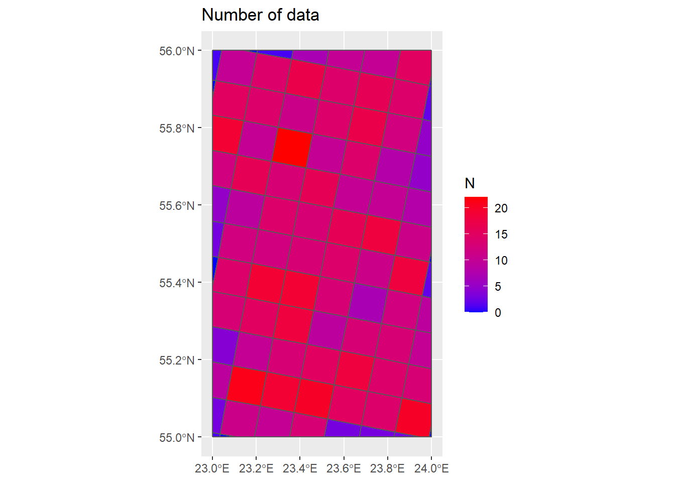
  ## Plot number of data in each grid cell ----
  cols <- colorRampPalette(c("blue", "red"))(6)
  P_Grids10km_N <- ggplot() +
    geom_sf(data = Country) +
    geom_sf(data = Grids_10km_Sum, aes(fill = N)) +
    scale_fill_gradient(low = "blue", high = "red") +
    ggtitle("Number of data")
  P_Grids10km_N
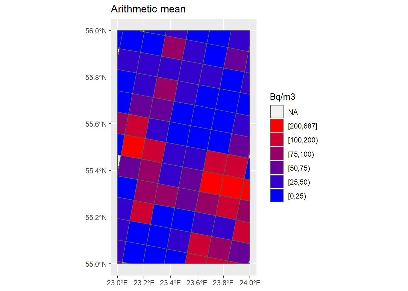
  ## Plot arithmetic mean ----
  max(Grids_10km_Sum$AM, na.rm = T)
# [1] 687
  breaks <- c(0, 25, 50, 75, 100, 200, max(Grids_10km_Sum$AM, na.rm = T))
  Grids_10km_Sum <- Grids_10km_Sum %>% mutate(AM_brks = cut(AM, breaks, include.lowest = T, right = F))
  cols <- colorRampPalette(c("blue", "red"))(6)
  P_Grids10km_AM <- ggplot() +
    geom_sf(data = Country) +
    geom_sf(data = Grids_10km_Sum, aes(fill = AM_brks)) +
    scale_fill_manual(name = "Bq/m3", values = cols, guide = guide_legend(reverse = TRUE)) +
    ggtitle("Arithmetic mean")
  P_Grids10km_AM
  ## Probabilistic maps ----
  # Probability of having an indoor radon concentration above the national reference level (e.g. RL = 200 Bq m-3)
  # Based solely on the indoor radon measurements in each grid of 10x10 km,
  # and assuming data independence and lognormality
  str(Grids_10km_Sum)
# Classes 'sf' and 'data.frame':    93 obs. of  17 variables:
#  $ CELLCODE  : chr  "10kmE512N371" "10kmE512N372" "10kmE513N366" "10kmE513N367" ...
#  $ EOFORIGIN : num  5120000 5120000 5130000 5130000 5130000 5130000 5130000 5130000 5130000 5130000 ...
#  $ NOFORIGIN : num  3710000 3720000 3660000 3670000 3680000 3690000 3700000 3710000 3720000 3730000 ...
#  $ Id        : Factor w/ 1022 levels "1","2","3","4",..: 340 341 361 362 363 364 365 366 367 368 ...
#  $ GID_0     : chr  "LTU" "LTU" "LTU" "LTU" ...
#  $ NAME_0    : chr  "Lithuania" "Lithuania" "Lithuania" "Lithuania" ...
#  $ N         : num  0 1 0 3 5 12 19 15 10 0 ...
#  $ Case      : num  NA 0 NA 0 1 0 0 0 0 NA ...
#  $ AM        : num  NA 5.11 NA 2.96 97.47 ...
#  $ SD        : num  NA NA NA 2.96 91.43 ...
#  $ GM        : num  NA 5.11 NA 2.06 56.42 ...
#  $ GSD       : num  NA NA NA 2.86 3.79 ...
#  $ MIN       : num  NA 5.113 NA 0.785 8.032 ...
#  $ MAX       : num  NA 5.11 NA 6.32 205.46 ...
#  $ geometry.x:sfc_POLYGON of length 93; first list element: List of 1
#   ..$ : num [1:4, 1:2] 23 23 23 23 55.9 ...
#   ..- attr(*, "class")= chr [1:3] "XY" "POLYGON" "sfg"
#  $ geometry.y:sfc_GEOMETRY of length 93; first list element:  list()
#   ..- attr(*, "class")= chr [1:3] "XY" "GEOMETRYCOLLECTION" "sfg"
#  $ AM_brks   : Factor w/ 6 levels "[0,25)","[25,50)",..: NA 1 NA 1 4 1 1 2 1 NA ...
#  - attr(*, "sf_column")= chr "geometry.x"
#  - attr(*, "agr")= Factor w/ 3 levels "constant","aggregate",..: NA NA NA NA NA NA NA NA NA NA ...
#   ..- attr(*, "names")= chr [1:15] "CELLCODE" "EOFORIGIN" "NOFORIGIN" "Id" ...
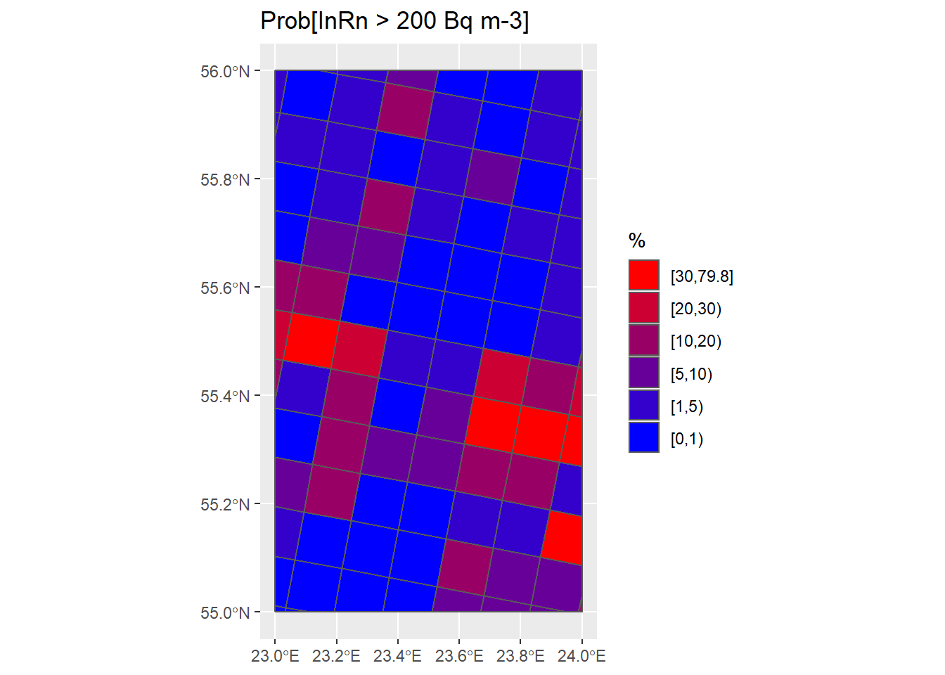
  # 1st: estimated Prob[InRn > 200 Bq m-3]
  RL <- 200
  Grids_10km_Sum <- Grids_10km_Sum %>%
    mutate(Prob = 100*(1-pnorm(log(RL), mean = log(GM), sd = log(GSD))))

  # 2nd: Replace values in grids with less than n data (i.e. N < 5) by a modeled value
  # Generate the points for the interpolation (centroid)
  DCen <- st_centroid(Grids_10km_Sum)
  # Inverse distance weighted (IDW) interpolation
  Prob_IDW <- idw(Prob ~ 1, filter(DCen, N > 5),
                  newdata = filter(DCen, N <= 5),
                  nmax = 10,
                  idp = 2 )
# [inverse distance weighted interpolation]
  # Replace values by the modeled values
  Grids_10km_Sum <- Grids_10km_Sum %>% mutate(Prob = replace(Prob, N <= 5, Prob_IDW$var1.pred))

  # Plot maps
  breaks <- c(0, 1, 5, 10, 20, 30, max(Grids_10km_Sum$Prob))
  Grids_10km_Sum <- Grids_10km_Sum %>% mutate(Prob_brks = cut(Prob, breaks, include.lowest = T, right = F))
  cols <- colorRampPalette(c("blue", "red"))(6)
  P_Grids10km_Prob <- ggplot() +
    geom_sf(data = Country) +
    geom_sf(data = Grids_10km_Sum, aes(fill = Prob_brks)) +
    scale_fill_manual(name = "%", values = cols, guide = guide_legend(reverse = TRUE)) +
    ggtitle("Prob[InRn > 200 Bq m-3]")
  P_Grids10km_Prob